
Computational pathology
Generating gastric tissue, from architecture to cells
How Grail combined tissue layout, public reference images and pathology diffusion to generate and measure synthetic gastric histology.
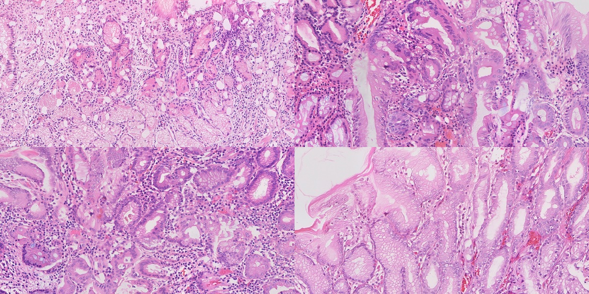
A histology image contains several kinds of information at once. From a distance, you see the arrangement of tissue: glands, open spaces, the mucosal surface. Closer in, you see cells and their nuclei. Closer still, a small cluster of organisms can change what the image means.
That makes generating one an interesting problem. The colours can look convincing before the anatomy does. A field can have plausible cells but put its glands in the wrong places. And a model that produces a convincing local patch still has to make those patches agree across a much larger field.
We built a system to explore this problem for the Singapore General Hospital synthetic histopathology challenge. Our starting idea was to give tissue arrangement and cellular appearance their own controls. A procedural model would describe the anatomy. A pathology-trained generator would render it. Measurements against real tissue would tell us what each part had actually contributed.
The most useful result was how differently those controls behaved. Matching real reference windows improved cellular appearance. Teaching the generator to read a tissue map gave it much stronger control over gland placement. Then a surprisingly small change to that map—removing separate nucleus channels—brought the nuclear statistics much closer to the real images.
This article follows those experiments through to the research collection: seventy synthetic fields, seventy public real reference fields, and ten synthetic images selected from the seventy for closer inspection. The technical report records the experiments in more detail.
What the image has to contain
The challenge centres on Helicobacter pylori and intestinal metaplasia. One asks us to represent small organisms in gastric tissue. The other asks us to represent a change in the epithelium, including mucin-rich goblet cells. Their co-occurrence adds another combination, and normal mucosa supplies the control.
Each field is a 4096 × 2048 RGB PNG. At the configured sampling of 0.25 micrometres per pixel, it covers 1.024 × 0.512 millimetres. That physical scale matters throughout the system. It connects the dimensions of a gland in the procedural model to the pixels in the output, and those pixels to the measurements we make later.
| Generation target | Selected ten | Synthetic collection |
|---|---|---|
| HP organisms with gastritis | 3 | 21 |
| Intestinal metaplasia | 2 | 14 |
| HP, gastritis and IM together | 2 | 14 |
| Normal control | 3 | 21 |
| Total | 10 | 70 |
Our normal tissue model has separate body and antrum presets. This is a useful example of why a category name alone is not enough: the same broad label can cover different arrangements of glands and pits. We wanted to be able to vary those arrangements deliberately.
Start with a piece of tissue
We began by constructing gastric mucosa in three dimensions. Hollow glands sit beneath a surface, surrounded by epithelium and lamina propria. Parameters set their diameter, wall thickness, pit depth and lumen shape. Other settings place stromal nuclei, inflammatory follicles and goblet-cell mucin.
A virtual section turns this volume into an image. Cut across a gland and it appears as a ring. Cut at an angle and the profile becomes oblique; cut along it and a channel appears. Changing the section gives us different views of the same underlying construction.
The section also produces a label map. Every pixel belongs to one of nine compartments: background, lumen, epithelial cytoplasm, goblet mucin, epithelial nucleus, stroma, stromal nucleus, vessel or red cell. This map gives the generator a spatial target and gives us something concrete against which to measure the result.
Some improvements happened before we used diffusion at all. The second version of the tissue renderer added epithelial granularity and a minimum gap between mucin and lumen. That kept the gland wall from turning into a row of disconnected mucin wedges. In the drawing evaluation, 68 of 72 category × cut × metric summaries fell within the real reference bands, compared with 50 of 72 for the earlier construction.
The tissue presets used in the experiments
These are the recorded v2 construction settings. They describe our implementation; the stromal counts are placement settings rather than measured densities in generated images.
| Parameter | Body | Antrum | Gastritis | IM | Mixed |
|---|---|---|---|---|---|
| Outer diameter, µm | 44–60 | 46–66 | 52–74 | 58–84 | 56–80 |
| Wall thickness, µm | 14–22 | 16–24 | 18–25 | 20–29 | 19–28 |
| Pit depth / slab depth | 0.22 | 0.42 | 0.50 | 0.28 | 0.38 |
| Goblet fraction | 0 | 0 | 0 | 0.36 | 0.30 |
| Stromal nuclei / mm² | 12,500 | 10,500 | 17,000 | 10,500 | 15,000 |
Give the drawing cellular appearance
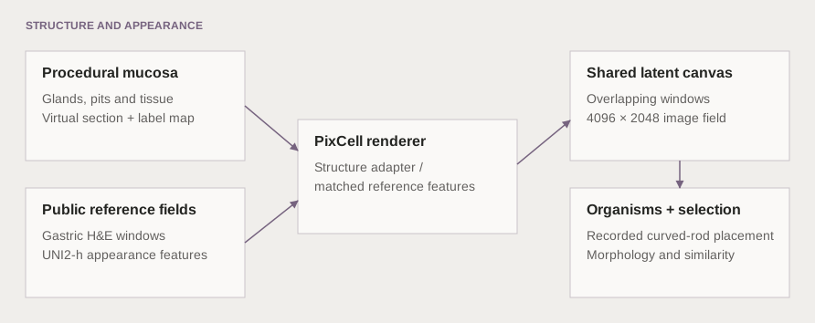
The next step was to render the tissue. We used PixCell-1024, a pathology diffusion transformer, with UNI2-h features from public reference images. UNI2-h represents each 1024-pixel reference window with sixteen appearance tokens. Those tokens give the renderer examples of how tissue looks.
We tried a single reference field, a mosaic of matched reference windows, and a trained structure adapter. The single-field route provided a useful baseline, though some of the reference architecture could persist. The mosaic allowed different parts of the output to draw on different real fields. The adapter added a direct route for the tissue map to influence the generator.
For the mosaic, we searched for a real window whose lumen and epithelial masks resembled the corresponding part of the synthetic drawing. This was a local choice: a gland-rich window could use one reference, while a neighbouring stromal window used another. A canvas used a median of eleven distinct reference fields, with a range of five to fourteen.
How reference matching and full-field rendering work
Each window searches 24 same-category training fields, 21 window origins and eight rotations or reflections: 4,032 candidates. The matching score is IoU(lumen) + 0.5 × IoU(epithelium), computed at one-eighth resolution using block-mean masks. IoU is the intersection of two masks divided by their union.
The full canvas uses 1024 × 1024 windows spaced 512 pixels apart. Seven horizontal origins and three vertical origins give 21 overlapping windows. Their denoising predictions are combined on the same latent canvas before decoding.
The adapter inference experiments used a 20-step DPMSolver++ schedule with classifier-free guidance of 1.5. We tested generation from noise and image-to-image repaint separately. Repaint start indices 6 and 3 leave fourteen and seventeen steps respectively.
The shared canvas is what makes the field larger than an individual rendering window. During denoising, overlapping windows contribute to the same representation. They have to agree in the overlap as the image develops. This gives neighbouring regions a common context instead of leaving the boundary problem until the image is finished.
Teach the model to read the map
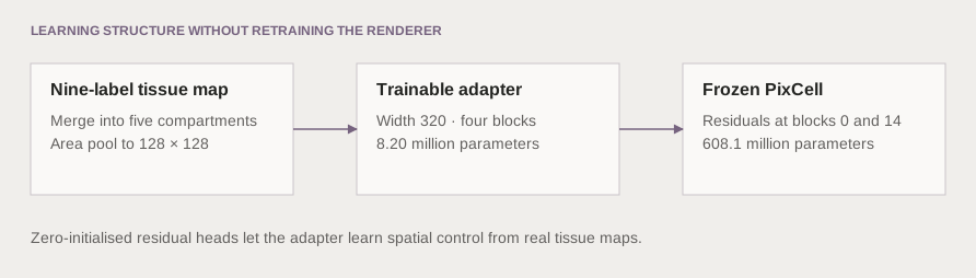
Reference matching could suggest a useful appearance, but it was an indirect way to request a shape. We therefore trained a small additional branch to read the tissue map and supply spatial guidance to the frozen generator. That branch is the structure adapter.
The first adapter, F2, received all nine labels. The next, F3, received five broader groups. Epithelial nuclei were merged into epithelium and stromal nuclei into stroma. The map still described where the main tissue compartments belonged, while the renderer had more freedom to produce their cellular detail.
Adapter architecture and training settings
F3 has width 320, four blocks and 8.20 million trainable parameters. Zero-initialised heads produce two spatial residuals, injected at blocks 0 and 14 of the 28-block, 608.1-million-parameter PixCell diffusion transformer. F2 has 8.25 million parameters. Setting the adapter scale to zero removes its residual contribution.
| Coarse channel | Labels combined |
|---|---|
| Background | Background above the surface |
| Lumen | Lumen |
| Epithelium | Cytoplasm, goblet mucin, epithelial nucleus |
| Stroma | Stroma, stromal nucleus |
| Vascular | Vessel, red cell |
Maps are area-pooled to 128 × 128. Each latent cell retains a soft partition whose channels sum to one. The checkpoint stores the grouping so inference reconstructs the same input vocabulary.
The 96-field development pool was split by slide into 64 training and 32 validation fields. This internal split is separate from the 22-field external morphometric calibration set. Training maps came from automatic segmentation of real images.
| Setting | Value |
|---|---|
| Crop and batch | 1024 pixels; batch size 4 |
| Training length | 3,000 steps |
| Learning rate | 10⁻⁴, cosine decay, 100 warmup steps |
| Regularisation | Weight decay 0.01; gradient clipping 1.0 |
| Dropout | Classifier-free and conditioning dropout, both 0.10 |
| Memory settings | bf16 and gradient checkpointing |
| Checkpoint / validation interval | 500 / 250 steps |
The coarse run completed in 8,198 seconds. Caching the model, reference tokens and label maps let a single inference process run many comparison jobs.
Add the smallest structures explicitly
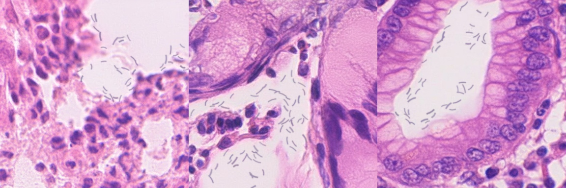
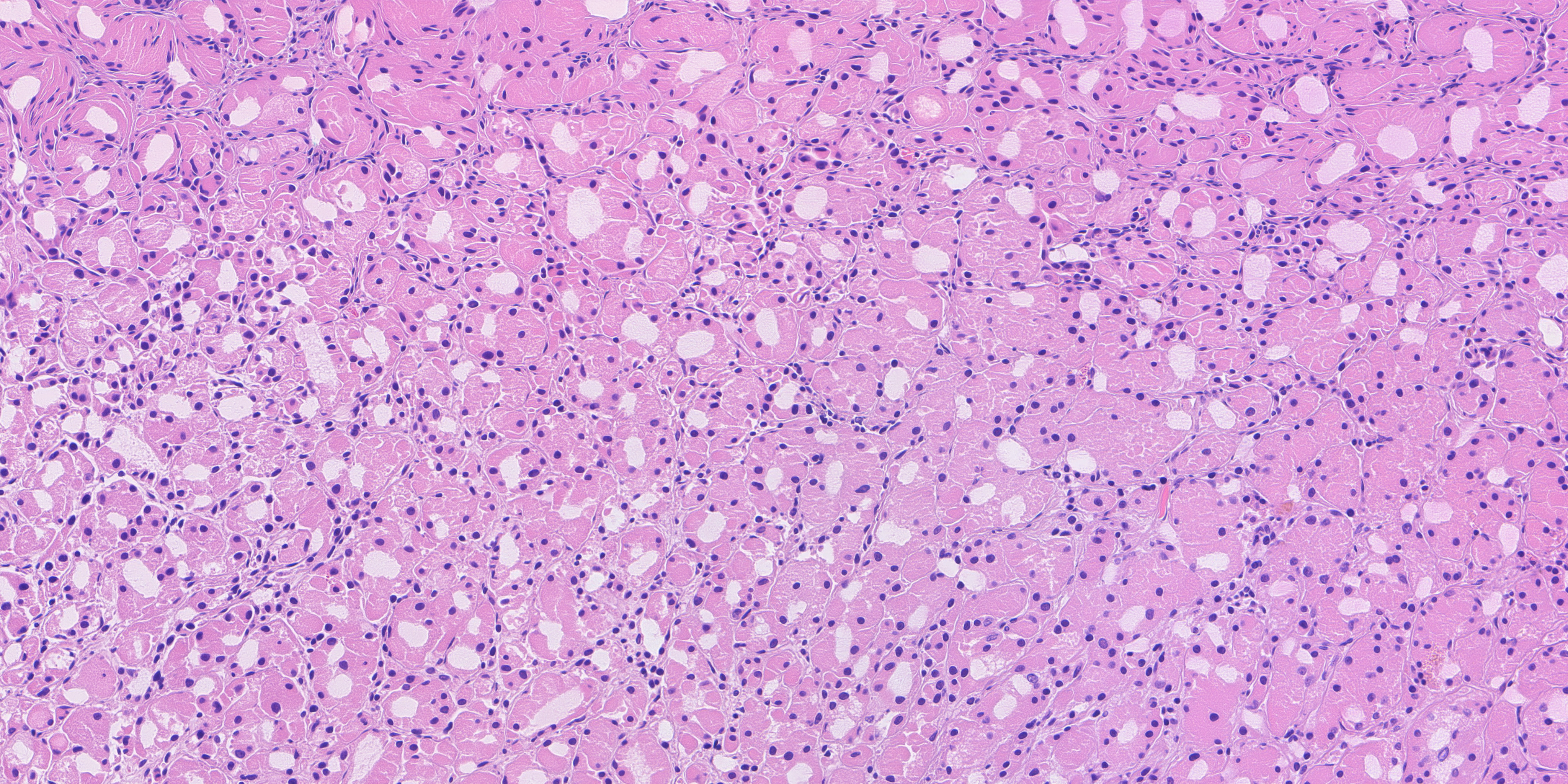
The HP-target images use a separate organism-rendering stage after diffusion. It places faint curved rods in surface mucus and pit or gland lumina, and records their positions, sizes and clusters. Across the five HP-target images in the final ten, it places 390 organisms, ranging from 48 to 90 per field.
Keeping that stage explicit makes the origin of the small structures clear. The tissue appearance comes from the diffusion model; the organism layer comes from procedural rendering, with its own placement record.
What changed when we changed the controls
To compare methods, we kept the requested drawings fixed. Otherwise, an easier drawing could make a weaker method look better. We measured both appearance and layout: how close the field was to real tissue in a morphometric feature space, and how closely its lumina followed the intended map.
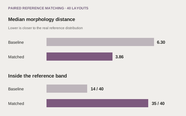
In the matched-reference experiment, A5, forty drawings covered four categories, five seeds and two cuts. Matching improved morphology distance on 37 of the forty pairs. The median fell from 6.30 to 3.86; the real held-out comparator was 3.51. The number inside the category reference band rose from fourteen to thirty-five.
But the generated lumina still followed the drawing weakly. Their overlap score, or IoU, rose from 0.0452 to 0.0835. Reference matching had helped the renderer find more suitable appearance without making it follow the requested geometry closely. That result made the case for direct structure conditioning much clearer.
The adapter experiments then exposed a second trade-off. Giving the adapter all nine labels produced strong layout control, but too many small nuclei. When we merged the nucleus labels into their surrounding tissue, nuclear density moved from 10,070 to 6,655 per square millimetre. The real comparator was 6,376. Median nuclear area moved from 17.6 to 24.2 square micrometres, against 23.1 in the real fields.
In relative terms, density error fell from about +58% to +4%, and area error from −24% to +5%. Lumen IoU fell from 0.466 to 0.395. We gave up some adherence to the drawing and gained substantially better cellular statistics.
| F3 comparison | Distance D | Lumen IoU | Nuclei / mm² | Median area, µm² |
|---|---|---|---|---|
| Real held-out, 22 fields | 3.51 | — | 6,376 | 23.1 |
| Two-pass repaint, si3 | 5.77 | 0.051 | 5,935 | 29.6 |
| F2 nine-channel, from noise | 9.03 | 0.466 | 10,070 | 17.6 |
| F3 coarse, from noise | 4.60 | 0.395 | 6,655 | 24.2 |
| F3 coarse, repaint si3 | 4.40 | 0.357 | 6,351 | 25.8 |
These are medians over the same twenty across-section drawings for the generated arms. They form a separate comparison from A5’s forty drawings.
We also tested whether the adapter itself caused the layout improvement. In twenty paired repaint runs, we held the drawing, starting image, donor, seed and seventeen-step schedule fixed, and changed only the nine-channel adapter scale. Turning it on increased lumen IoU by a median 0.434 and ring IoU by 0.271. The adapter-off medians were 0.051 and 0.045. The extra layout control came with a median increase of 1.30 in morphology distance.
Together, these experiments explain the direction of the work. Appearance matching is useful. Spatial guidance is useful. The better system has to let us control both, and measure what we lose when we improve one.
Choosing the final collection
The same lesson carried into selection. Minimising a single distance score can favour familiar texture while losing an anatomically useful view. We ranked the original ten and seventy together, then inspected leading candidates as complete fields and at native-pixel scale.
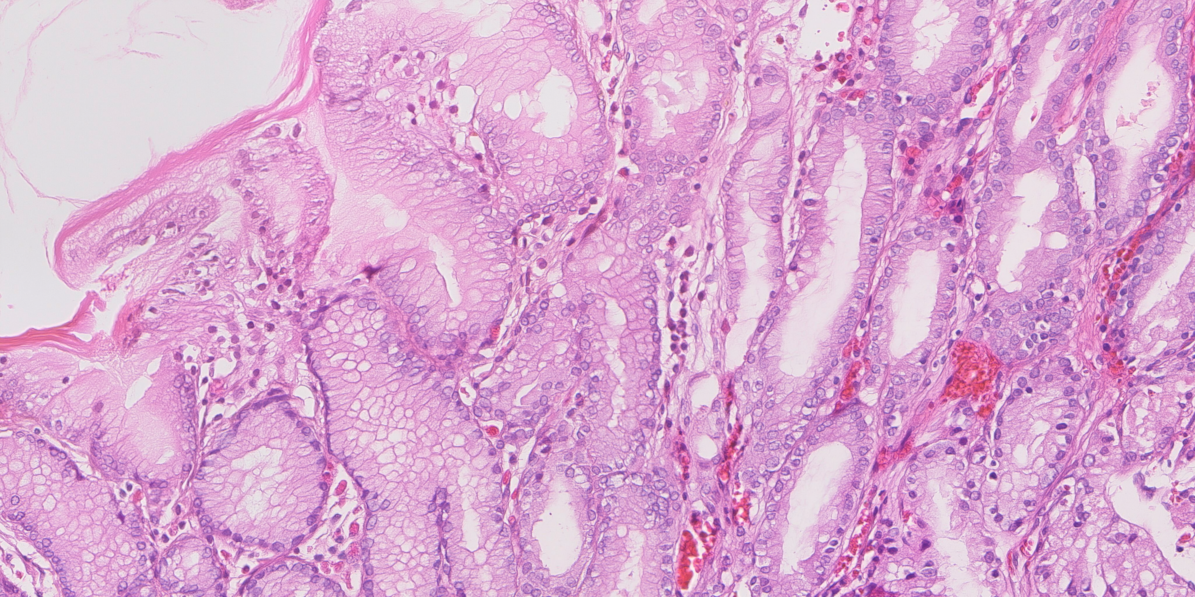
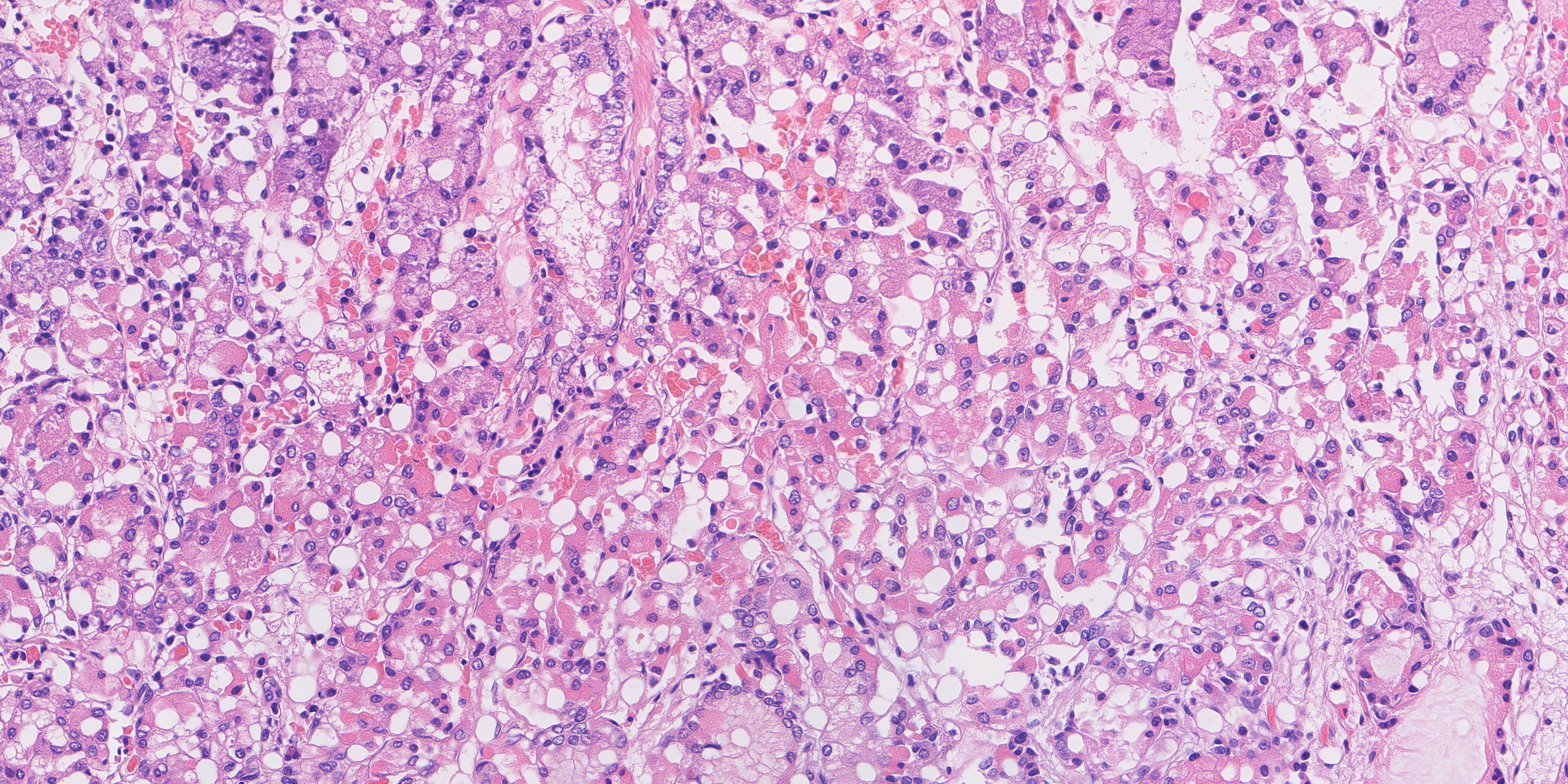
The final choice keeps the strongest measured HP and mixed examples, favours an IM field with clearer epithelial detail, and includes a normal view running from the surface into the glands. All three normal fields fall within the original gland-ring range. Their inclusion raises the average distance slightly compared with a choice made only by that score, but preserves more useful anatomy.
| Final-ten measurement | Value |
|---|---|
| Mean morphology distance | 3.189 |
| Normal gland-ring fractions | 0.816 · 0.717 · 0.733 |
| Original normal ring range | 0.671–0.976 |
| Minimum recorded embedding-copy margin | 0.0532 |
| Maximum recorded pixel NCC | 0.8219 |
| Procedural organisms in HP-target fields | 390 |
The ten are contained in the final seventy. Across the seventy, we checked all 602 same-category pairs at two resolutions. Maximum SSIM was 0.5671 at 128-pixel width and 0.7053 at 1024-pixel width, below the 0.75 repetition threshold. The final ten use eight mosaic-conditioned examples, one procedural-layout example and one single-field-conditioned example.
The selected ten
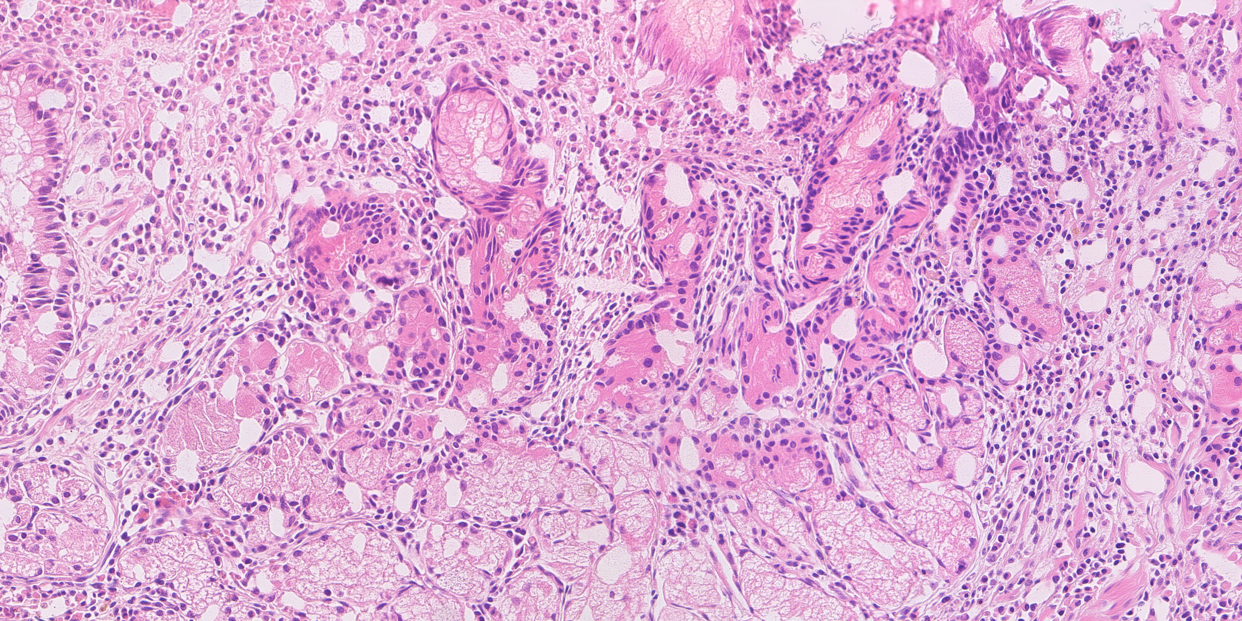
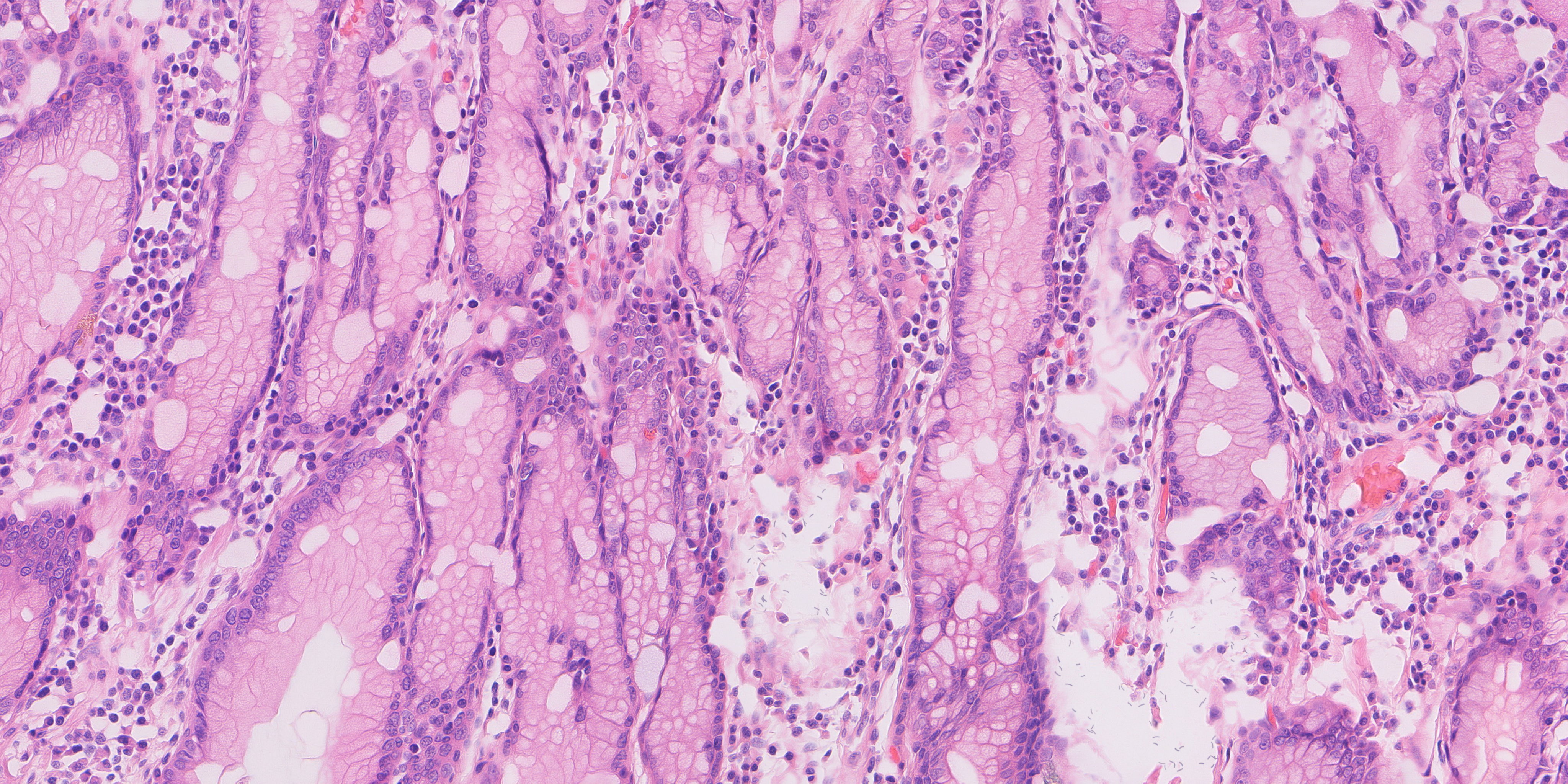
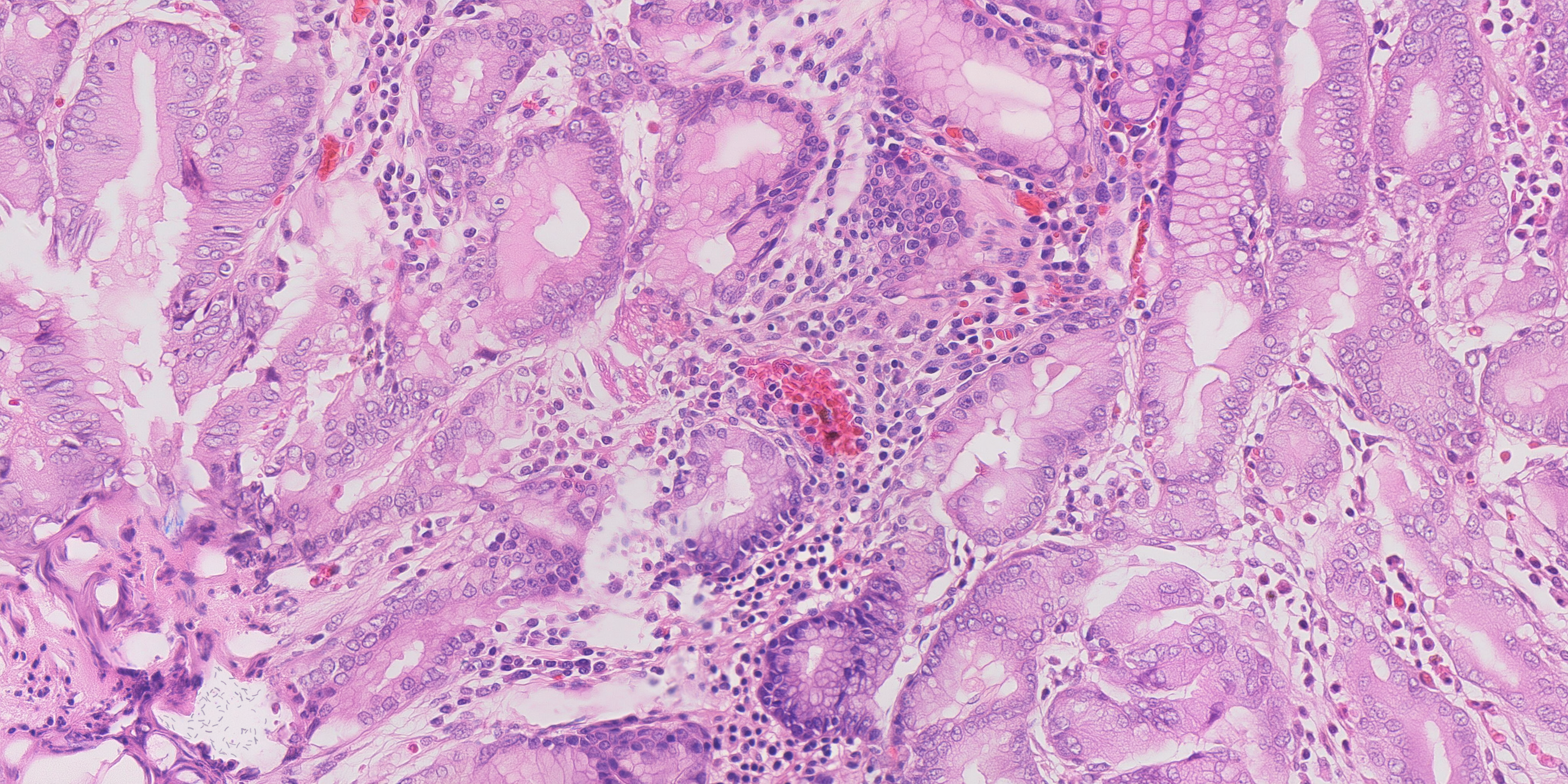
The images below are previews of the final fields. Each opens the full 4096 × 2048 PNG, where the smaller structures can be examined at their actual pixel size.
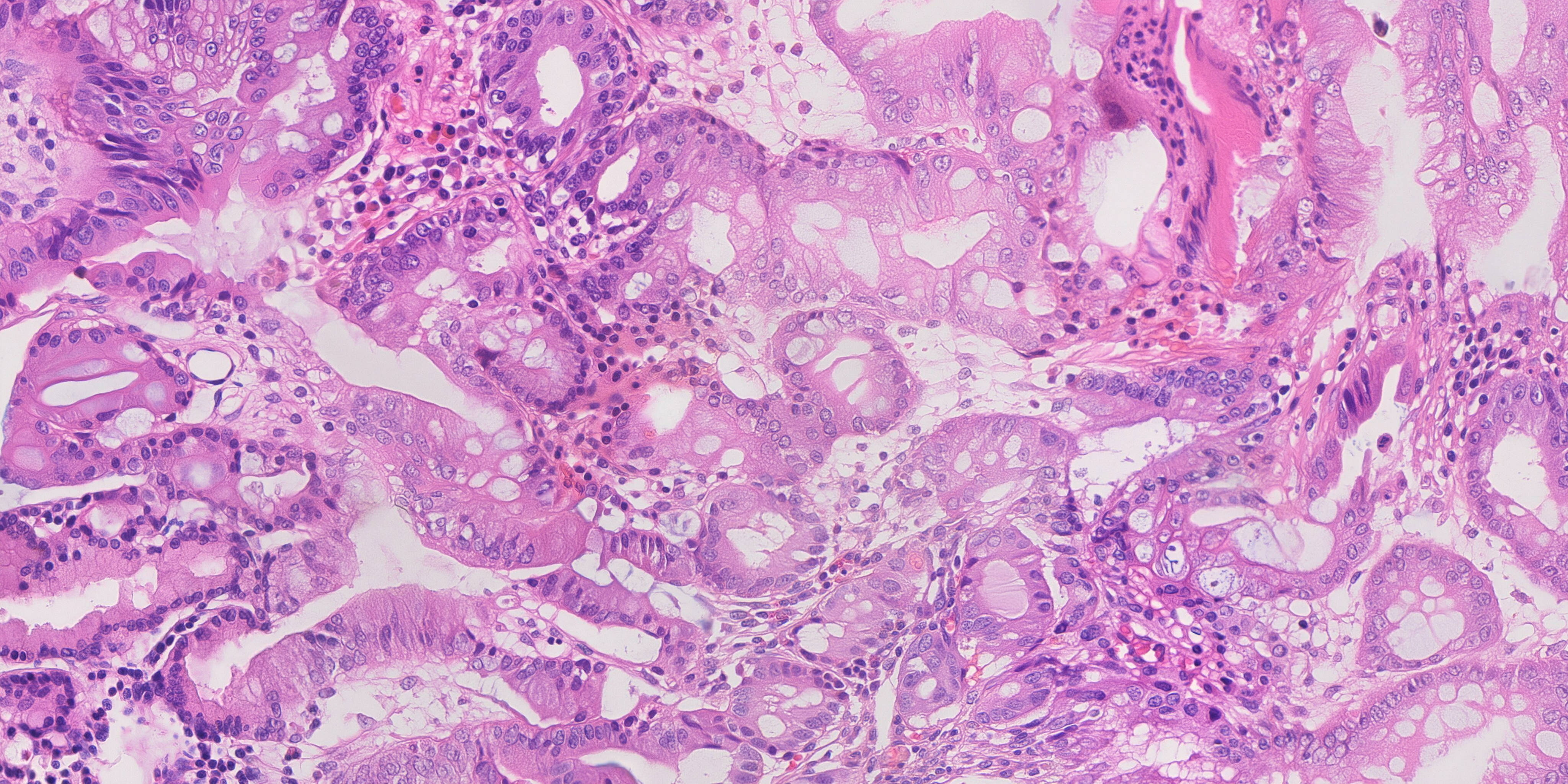
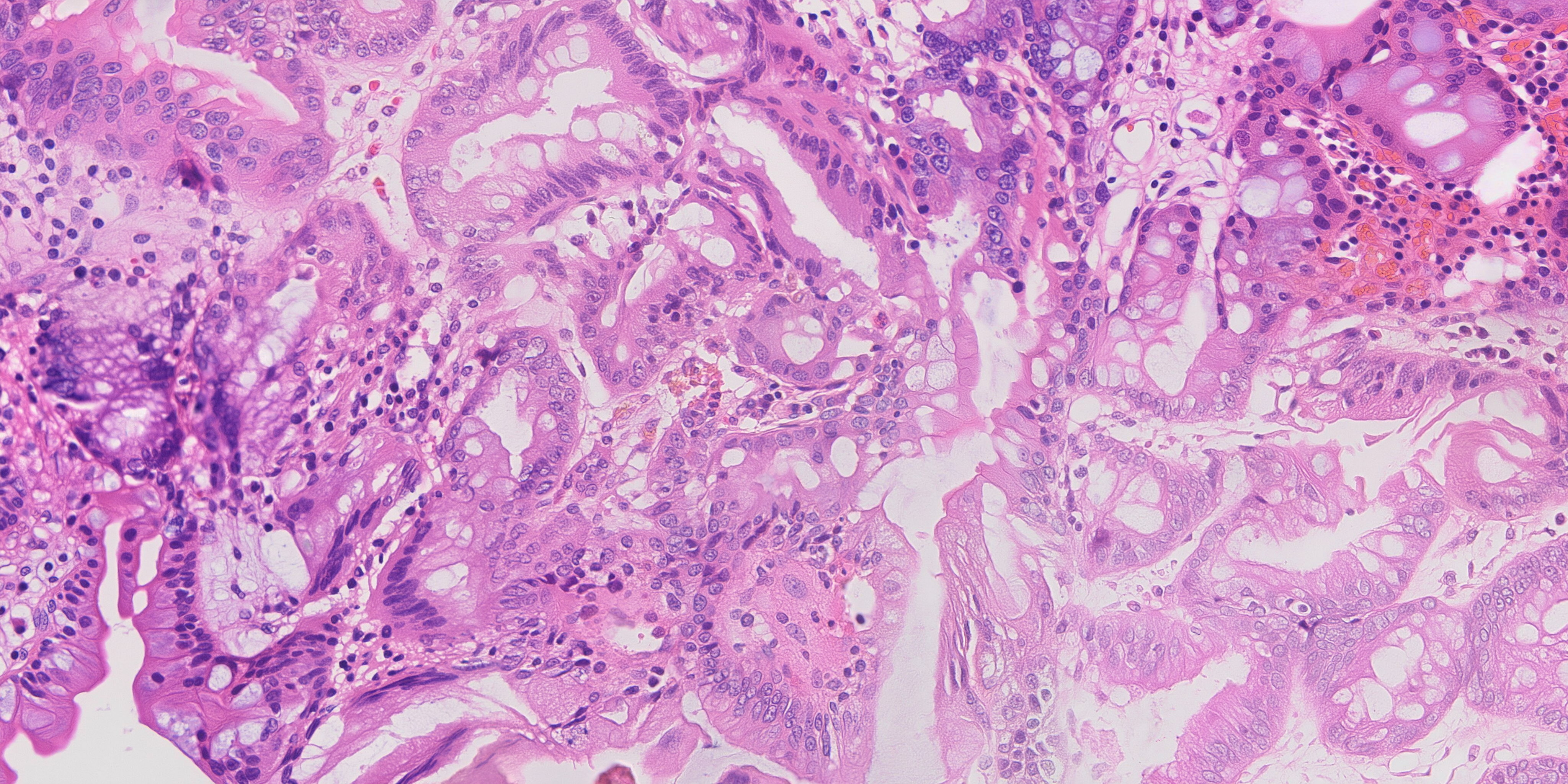
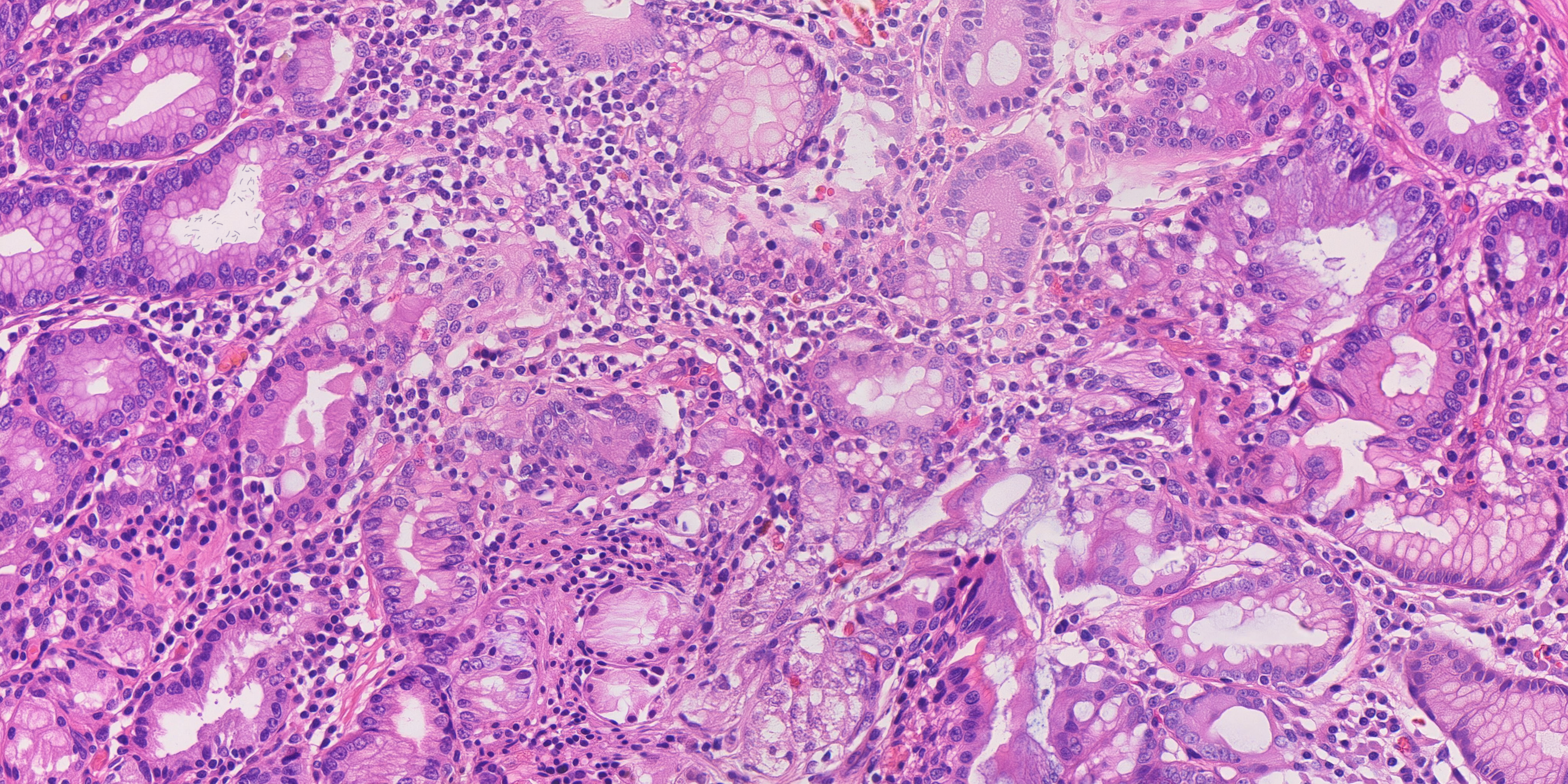
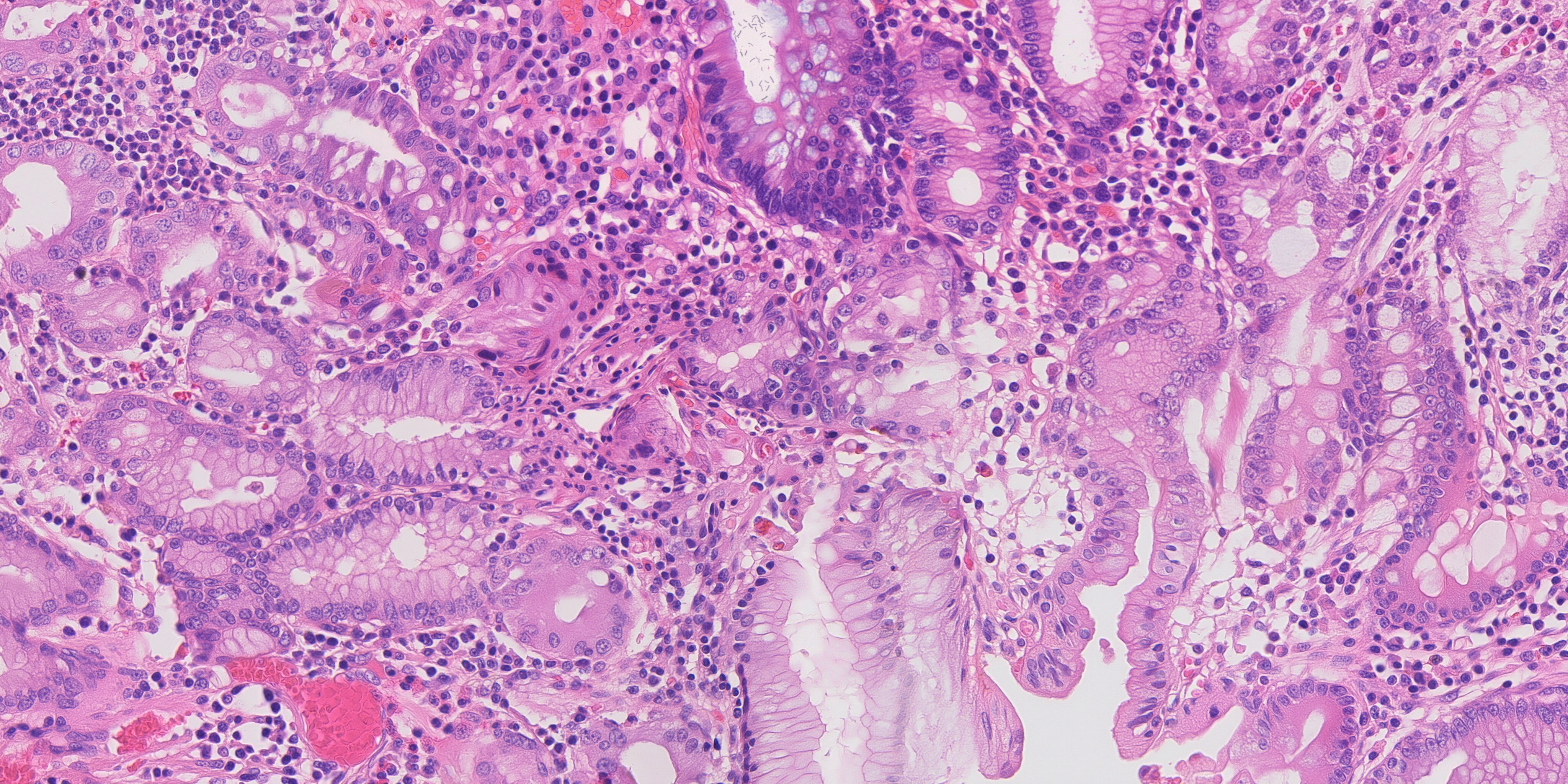
What the public data gives us
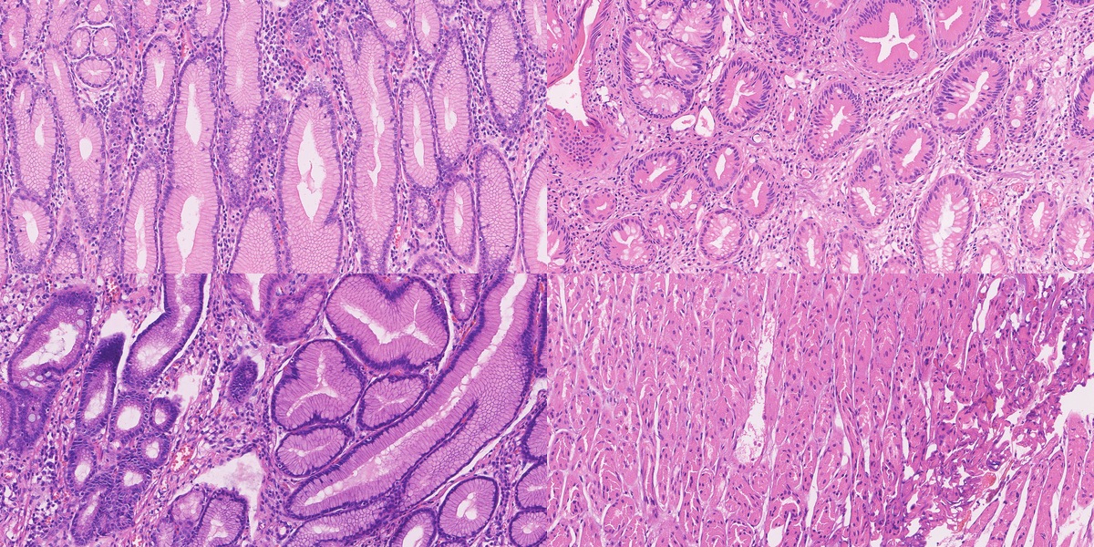
The work begins with real tissue. Our main high-resolution source is HiESD, a gastric whole-slide dataset with region annotations. Its full release contains 104 slides from 44 patients. Our seventy real reference fields come from nineteen slides, with no more than four fields per slide.
For that collection, we extracted 4166 × 2083 pixels at the original sampling of 0.2458 µm per pixel and downsampled to 4096 × 2048 at approximately 0.25 µm per pixel. Each field retains its source slide and extraction rectangle. A slide is large enough to provide several fields, so seventy images here means seventy tissue regions, rather than seventy independent specimens.
We also extracted and inspected GasHisSDB, which contains 245,196 patches. Its size is attractive, but the patches are only 80, 120 or 160 pixels square. They show local texture. A whole-slide region shows how that texture fits into a larger piece of anatomy. Both can be useful if we give them the right role.
| Public resource | Size | Role |
|---|---|---|
| HiESD | 104 whole slides | Gastric architecture, scale and region annotations |
| GasHisSDB | 245,196 small patches | Local texture and stain variation |
| GastritisMIL public release | 800 whole slides | Further antral and corpus biopsy morphology |
| Public H&E figures and educational micrographs | Curated by source | Localized organism examples and descriptive context |
Enlarging a small patch does not reveal more tissue. Our training plan therefore keeps small-patch texture learning separate from native-scale field learning. It also keeps the source annotation intact. A normal-gland region is an annotation of that region; a chronic-gastritis label does not supply an HP organism label.
How we measure the result
Once a generator can produce plausible-looking tissue, it becomes easy to argue about examples. We wanted a way to compare runs systematically. The measurement instrument describes gland topology, nuclear morphology, epithelial spacing, stromal texture, stain and tissue fractions.
It reports 54 values. The main distance, D, uses ten core features and accounts for how those features vary together in real tissue. A separate diagonal summary uses 33 standardised features. Keeping these distinctions explicit matters: “54 measurements” does not mean that every value contributes to the same score.
Calibration used 96 public reference fields, twenty-four per programme category, and a further twenty-two fields held out by slide. A generated field is “inside the band” when its D is at or below the largest held-out value for that category. It is a comparison of measured morphology. Disease annotations remain a separate part of the record.
Feature extraction, distance calculation and calibration
Images are analysed at 1536 × 768, an effective sampling of 0.6667 µm per pixel. Optical density is OD = −log((RGB + 1) / 256). Fixed H&E stain vectors retain stain shifts in the measurements. Watershed splits nuclear candidates, which are filtered to areas of 5–180 µm². The epithelial proxy uses a 6 µm morphological closing of the haematoxylin-rich mask.
For 33 selected features, robust standardisation is z = (x − median) / (1.4826 × MAD), with standard-deviation fallback. Their root mean square forms the diagonal summary.
D is a robust Mahalanobis distance using gland-hole fraction, ring density, nuclear density and median area, epithelial nearest-neighbour distance and its coefficient of variation, stromal orientation coherence and eosin variance, and mean H and E optical density. MinCovDet uses a support fraction of 0.75 and a ridge of 0.10 times the mean covariance diagonal.
| Category | Training / held out | Median D | Maximum D |
|---|---|---|---|
| Normal | 24 / 4 | 3.33 | 4.34 |
| Gastritis | 24 / 6 | 4.19 | 7.97 |
| IM | 24 / 6 | 2.58 | 4.50 |
| Mixed | 24 / 6 | 3.66 | 4.38 |
These are empirical ranges from the stated calibration fields. Native-pixel inspection complements the downsampled instrument, particularly for small organisms and other fine detail.
We also ask how similar a generated image is to its references. A pathology encoder finds nearby reference tiles; a pixel-correlation search then examines source fields and embedding neighbours. That lets us inspect source influence at two levels. Tissue arrangement needs its own comparison, because it can persist even when the pixels differ.
The similarity screen recorded in the technical report
The earlier screen ran after procedural organism rendering. It compared eighty candidate tiles with 944 tiles from 118 reference fields using phikon-v2. Maximum cosine similarity was 0.8995, below its 0.95 flag threshold.
The pixel screen covered 83 candidate/reference pairs and 10,568 search windows, using 64-pixel patches with stride 256. Maximum normalised cross-correlation was 0.7889, below 0.92. The search included token-source fields and nearest neighbours found by the embedding screen. These are the report's earlier screen results; the final-ten measurements are given above.
The earlier selection also contained one normal gland-hole fraction of 0.985, above the 0.976 reference maximum. The final selection replaces that case: all three normal fractions are now within the original range.
The record of an image is part of the output. It links the map and source hashes, window origins and transforms, generation route, seed, scheduler, adapter and label grouping to the final PNG. Measurements and organism-placement records attach to that image’s checksum. A result can therefore be traced back to the field that was actually generated and measured.
The next useful test follows from the purpose of the challenge. Train an anomaly detector on real images, then train the same detector on real plus synthetic images, and compare them on independent real cases. Sensitivity, specificity, performance by category and variation across slides will show which synthetic examples help. The generation measurements give us a way to improve candidates; that downstream experiment will tell us how much those improvements matter.
OIP technical report · 8 pages
Final executive summary · Selected-ten measurements · Ten-to-seventy mapping
Your software should be moving faster.
Show us what is stuck. We’ll tell you what we would take over first and how we would get delivery moving again.